
Even though Microsoft Excel has been around for almost three decades, it’s still the gold standard.
With its multitude of features and functions, you can organize, visualize, collate, combine and even forecast all sorts of data with just a few clicks or a formula or two.
Whether you’re an Excel novice or veteran, the 23 tips and tricks in this article will help you make the most out of this “oldie but goodie” and take your productivity to the next level:
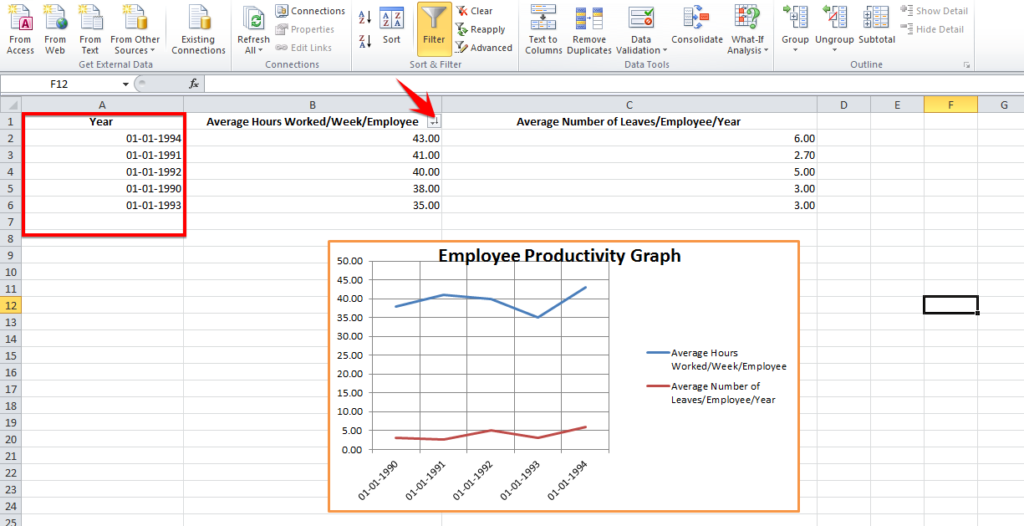
1. Charts and Graphs
With Excel, you can create visuals such as charts and graphs to illustrate how the numbers on your spreadsheet relate to each other, help your readers process the information faster, and increase retention rate by as much as 400%.
Excel has a variety of built-in chart and graphs for you to choose from. After you’ve created a basic graph, you can use the “design” “layout” and “format” tabs under “chart tools” to refine your layout.
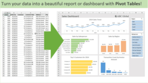
2. Pivot Tables
Do yourself a favor and learn pivot tables. It’s arguably the most powerful feature in Excel. What can you do with it? Quickly summarize a large amount of data into lists and tables…without writing a single formula.
Go to Insert > Pivot Table and select your data range. Then base on your needs, you can proceed with either “recommended pivot table” or manually create one:
3. Power View
This feature helps you take your data from the back office to the boardroom by collating and analyzing large datasets to create interactive, presentation-ready reports compatible with MS PowerPoint.
Simply turn on the Power View add-in and the button will show up on your toolbar.
4. VLOOKUP
If you frequently work with data across multiple Excel spreadsheets, VLOOKUP will become your new best friend (if it isn’t already.)
This feature allows you to collect data from different sheets and workbooks, and then bring it together to generate reports and summaries.
Go to File > Formula and enter the cell that contains your reference number to utilize this function.
5. Index Match
Similar to VLOOKUP, INDEX MATCH helps you pull data from other datasets into one central location.
VLOOKUP only works as a left-to-right lookup so if you need to do a right-to-left one, you’d have to rearrange those columns – a task which is not only tedious but also error-prone.
If you’re combining data from sources in which the columns don’t correspond, you can use INDEX MATCH so you don’t have to switch the columns around.
INDEX MATCH is a much more complex function than VLOOKUP so if you’re dealing with large datasets the load time could get slowed down.
6. Combining Cells
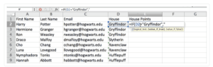
You can combine information from different cells into one cell. To do this, use the “&” sign in your function to streamline or simplify the data – e.g. =A2&” “&B2.
This can be helpful when dealing data such as names and addresses that tend to get broken up into many individual cells when imported into Excel.
How to Make a Graph in Excel & Add Visuals to Your Reporting
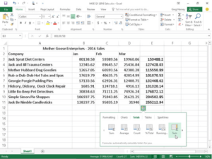
7. Quick Analysis
This tool helps you work with a small dataset so you can quickly generate charts, tables and graphs.
Select the cells and then click the Quick Analysis tool that automatically appears in the lower-right corner of the bottom of the selection:
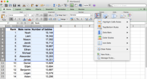
8. Conditional Formatting
With this function, you can automatically highlight points of interest within your dataset by setting the condition for which the cells would be formatted differently (e.g. filled with a different color) when the data meets (or does not meet) certain criteria.
Go to Home > Conditional Formatting > Add to set up a conditional formatting.
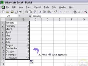
9. Autofill
Excel can recognize patterns within your dataset and fill in rows or columns automatically, saving you a considerable amount of time.
To use this feature, simply click on a cell, hold down the lower-right corner and drag down the column:
10. Apply Formula Down the Entire Column (without pasting 400 times)
When you input a formula in a cell, you can double-click the lower right of the cell and have the formula repeated in each of the cells down the column.
Alternatively, you can go to Fill > Down and have the formula populated down the entire column.
11. Excel Text-To-Speech
You can get Excel to repeat the numbers or data back to you to check for errors as you type.
You can activate this feature by clicking on More Commands > All Commands > Speak Cells to add this function to your quick access toolbar.
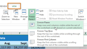
12. Freeze Panes
To keep the column or row names static while you scroll through the data, you can freeze the panes to help keep track on the data you’re looking at.
To freeze panes, click on the cell below the column heading and to the right of the label for each row, then to go View > Freeze Panes > Freeze Panes to make the column headings stay still so you can see them at all times.
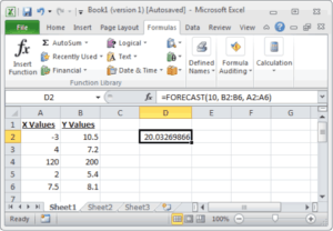
13. Make Projections
You can find a trend and predict values based on the data in your worksheet using the Forecast feature in Excel.
This feature can help project future sales, inventory requirements, or consumer trends.
To do so, apply the FORECAST function syntax =FORECAST(x, known_y’s, known_x’s) as a formula to the cell:
https://www.workzone.com/blog/excel-project-management-tool/
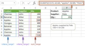
14. SUMIFS Function
This function sums cells in a range that match the supplied criteria. It can be used to sum values when adjacent cells meet criteria based on dates, numbers, and text.
It’s represented by the syntax =SUMIFS (sum_range, range1, criteria1, [range2], [criteria2], …)
This function sums cells in a range that match the supplied criteria. It can be used to sum values when adjacent cells meet criteria based on dates, numbers, and text.
It’s represented by the syntax =SUMIFS (sum_range, range1, criteria1, [range2], [criteria2], …)
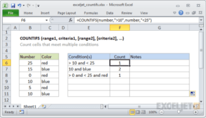
15. COUNTIFS Function
The COUNTIFS function applies criteria to cells across multiple ranges and counts the number of times all criteria are met.
It’s represented by the syntax =COUNTIFS(criteria_range1, criteria1, [criteria_range2, criteria2]…)
16. IF-THEN Statement
Using the IF THEN Excel formula (=IF(logical_test, value_if_true, value of false), you can set conditions for data to be inserted based on conditions.
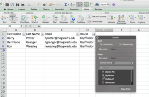
17. Filtering
This feature helps pare down your data and show rows that fit into certain criteria.
To access the feature, go to Data > Filter. Click the arrow next to the column headers to choose between ascending or descending order, as well as which specific rows to show.
18. Transpose
Let’s say you want to turn data in a column into a row, or vice versa. Just the thought of cutting and pasting each cell to reorder everything would make you want to cry.
Luckily, you can use the transpose function: highlight the column you want to transpose into rows. Then Copy > Paste Special > Transpose and you’re done!
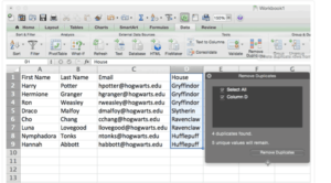
19. Remove Duplicates
This feature is particularly handy when you’re dealing with larger datasets that come from multiple sources – e.g. contact lists.
To use this function, highlight the row or column you want to remove duplicates from. Then go to Data > Remove Duplicates and you’re all set.
20. Absolute Formula
Most people use relative formulas (e.g. (=A5+B5)) in which the values will adjust based on where they’re moved if they’re copied-and-pasted from one cell to another.
If you want the values to stay the same no matter whether they’re moved around or not, you can use an absolute formula in which the exact column and row are held the same even if you copy the same formula into adjacent rows.
To set up an absolute formula, add the dollar sign before the numbers and alphabets representing the cell’s row and column, e.g. (=$A$5+$B$5).
21. Deleting Blank Cells
When you import data, you might get blank cells that’d impact the accuracy of your calculation. To quickly delete all blank cells, you can select the column and go to Data > Filter. In the dropdown menu, undo Select All and then check the box next to “Blanks.” You’ll now be able to see all the blank cells and delete them all at once.
22. Data Validation Function
You can use the data validation function to exclude invalid input by restricting input value in a column. You can weed out invalid data before it has the chance to get onto your spreadsheet.
To use this function, go to Data > Data Validation >Setting and input the conditions.
You can also shift to Input Message and set up prompts such as, “Please input your age with whole number, which should range from 18 to 60.” Users will get this prompt when hovering the cursor in this area and get an error message if the inputted information is unqualified.
23. “Shortcut” For Inputting Complicated Terms
It’s tedious and time-consuming to enter long phrases or complicated terms multiple times.
You can create “shortcuts” by using the autocorrect function: go to File > Options > Proofing > AutoCorrect Options. Enter your “shortcut” in the “Replace” box and the complete phrase or term in the “With” box.
There you have it – 23 tips and tricks to help you become faster and more productive with Microsoft Excel!